|
|
| |
|
| ||
|
|
| |
|
| ||
Dans cette partie, toutes les fonctions sont supposées définies sur un ouvert ![]() de
de ![]() .
.
On travaillera toujours sur ce domaine ![]() , sur lequel on a donc une application.
, sur lequel on a donc une application.
Définition : ![]() , définie sur
, définie sur ![]() , un ouvert de
, un ouvert de ![]() ,
,
on appelle dérivée partielle de![]() par rapport à la
par rapport à la ![]() variable, au point
variable, au point ![]()

si cette limite existe.
Sinon, on dit que ![]() n'admet pas de dérivée partielle par rapport à la
n'admet pas de dérivée partielle par rapport à la ![]() variable, au point
variable, au point ![]() .
.
On parle parfois de dérivée partielle première.
Remarque : Quand il n'y a que 2 ou 3 variables on note souvent les dérivées partielles,

Mais, on n'oubliera pas, en cas d'ambiguïté, qu'il s'agit des dérivées par rapport à la première, la seconde, ou la ![]() variable...
variable...
Définition : ![]() est de classe
est de classe ![]() sur
sur ![]() un ouvert de
un ouvert de![]() admet
admet ![]() dérivées partielles continues sur
dérivées partielles continues sur ![]() .
.
C'est à dire :  est définie et continue sur
 ![]()
Définition : ![]() , définie sur
, définie sur ![]() , un ouvert de
, un ouvert de ![]() , de classe
, de classe ![]() sur
sur ![]() , on appelle différentielle de
, on appelle différentielle de ![]() en
en ![]() , l'application linéaire notée
, l'application linéaire notée ![]()
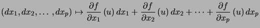
noté le plus souvent, pour alléger les notations : 
Dans le cas de 2 ou 3 variables, on note souvent la différentielle de ![]() en
en ![]()

ou bien : 
Théorème : ![]() , définie sur
, définie sur ![]() , un ouvert de
, un ouvert de ![]() , de classe
, de classe ![]() sur
sur ![]() ,
, ![]() .
.![]() admet un développement limité à l'ordre 1 en
admet un développement limité à l'ordre 1 en ![]() et
et
![]() avec
avec 
C'est à dire pour 3 variables par exemple :

Preuve. On le montre pour 3 variables. La démonstration repose sur le théorème des accroissements finis.
Pour cela, il faut faire varier les variables une à la fois.
|
|
|
|
|
|
|
|
|
|
|
|
|
|
|
avec ![]() .
.
D'où, par continuité des dérivées partielles :
|
|
|
|
|
|
Il ne reste qu'à regrouper les ![]() en un seul
en un seul![]() .
. ![]()
Définition : ![]() , définie sur
, définie sur ![]() , un ouvert de
, un ouvert de ![]() , de classe
, de classe ![]() sur
sur ![]() ,
, ![]()
On appelle gradient de ![]() en
en ![]() , noté
, noté ![]() le vecteur :
le vecteur : ![\begin{displaymath}\left( \begin{array}[c]{c} \dfrac{\partial f}{\partial x_{1... ...artial f}{\partial x_{p}}\left( u\right) \end{array} \right) \end{displaymath}](img56.png)
Ce gradient a une grande importance dans l'étude des courbes d'équation ![]() ou des surfaces d'équation
ou des surfaces d'équation![]() dans un repère orthonormal.
dans un repère orthonormal.
Définition : ![]() , définie sur
, définie sur ![]() , un ouvert de
, un ouvert de ![]() , de classe
, de classe ![]() sur
sur ![]() ,
, ![]()
On appelle dérivée de ![]() suivant le vecteur
suivant le vecteur![\begin{displaymath}\overrightarrow{V}:\left( \begin{array}[c]{c} v_{1}\\ v_{2}\\ \vdots\\ v_{p} \end{array} \right) \end{displaymath}](img59.png) en
en ![]() le produit scalaire
le produit scalaire

Théorème : L'ensemble des applications de classe ![]() sur
sur ![]() un ouvert de
un ouvert de ![]() , à valeur réelle, muni de
, à valeur réelle, muni de ![\begin{displaymath} % latex2html id marker 3963 \left\{ \begin{array}[c]{c} \t... ... \text{Le produit de deux applications} \end{array} \right\} \end{displaymath}](img62.png) a une structure d'algèbre commutative.
a une structure d'algèbre commutative.
Preuve. On montre que c'est une sous-algèbre de ![]() . Clairement,
. Clairement, ![]()
![]()
On écrit le théorème pour une fonction de 3 variables. L'énoncé pour une fonction de ![]() variables s'en déduit facilement.
variables s'en déduit facilement.
Théorème : ![\begin{displaymath}\left. \begin{array}[c]{r} x, y, z:\mathbb{R}\rightarro... ...), y(t), z(t)\right) \end{array} \right\} \Rightarrow F\end{displaymath}](img64.png) est de classe
est de classe ![]() sur
sur ![]() , et :
, et :

Ou encore, en utilisant la notation différentielle : 
Bien sûr, toutes les dérivées partielles sont prises en ![]() et les dérivées en
et les dérivées en ![]() .
.
Preuve. On écrit la démonstration pour une fonction de 2 variables seulement !
|
|
|
|
|
|
|
|
|
|
|
|
|
|
|
|
|
|
![]()
Théorème : On écrit ce théorème pour la composée de fonctions de plusieurs variables avec 2 et 3 variables.
Ceci est bien sûr arbitraire, le théorème s'applique avec ![]() et
et ![]() variables...
variables...![\begin{displaymath}\left. \begin{array}[c]{r} f:\mathbb{R}^{3}\rightarrow\math... ...) , w\left( x, y\right) \right) \end{array} \right. \quad\end{displaymath}](img78.png) est de classe
est de classe ![]() sur
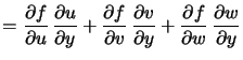
sur ![]() et :
et :
|
|
|
|
|
|
On a aussi changé les notations parce qu'il faut pouvoir s'adapter !
Preuve. Quand on fixe ![]() , on se retrouve exactement dans les hypothèses du théorème précédent.
, on se retrouve exactement dans les hypothèses du théorème précédent.
Ce qui donne ![]() . De même, on fixe
. De même, on fixe ![]() pour obtenir
pour obtenir ![]() .
. ![]()