|
|
| |
|
| ||
|
|
| |
|
| ||
Définition : ![]()
![]() , définie sur
, définie sur ![]() un intervalle de
un intervalle de ![]() . avec :
. avec : ![]() qu'on notera en ligne ou en colonne selon les cas.
qu'on notera en ligne ou en colonne selon les cas.
On dit que ![]() est de classe
est de classe ![]() sur
sur ![]() sont de classe
sont de classe ![]() sur
sur ![]()
On note d'ailleurs, pour ![]() :
: ![]() ou simplement :
ou simplement : ![]()
On fait de même pour les dérivées d'ordre supérieur.
Théorème : ![]() , l'ensemble des applications de classe
, l'ensemble des applications de classe ![]() définies sur
définies sur ![]() , à valeur dans
, à valeur dans ![]() , muni
, muni
est un espace vectoriel sur ![]() .
.
Preuve. C'est encore une fois clairement un sous espace vectoriel de ![]() .
. ![]() est bien non vide (application nulle) et stable par combinaison linéaire.
est bien non vide (application nulle) et stable par combinaison linéaire.
Il suffit d'appliquer le théorème pour les applications à valeur réelle à chaque coordonnée. ![]()
Définition : On dit que ![]() admet un développement limité à l'ordre
admet un développement limité à l'ordre ![]() en
en![]()
![]() chacune des
chacune des ![]() coordonnées de
coordonnées de ![]() admet un développement limité à l'ordre
admet un développement limité à l'ordre ![]() en
en ![]() .
.
Théorème : ![]() de classe
de classe ![]() au voisinage de
au voisinage de ![]() admet un développement limité d'ordre
admet un développement limité d'ordre ![]() au voisinage de
au voisinage de ![]() .
.
De plus, on a

avec ![]() quand
quand ![]()
On notera que ![]() et
et ![]() sont des fonctions vectorielles.
sont des fonctions vectorielles.
Cette formule s'appelle encore formule de Taylor-Young à l'ordre ![]() .
.
Preuve.![]() est de classe
est de classe ![]() au voisinage de
au voisinage de ![]() , d'où chaque
, d'où chaque![]() est de classe
est de classe ![]() au voisinage de
au voisinage de ![]() .
.
Chaque![]() admet donc un
admet donc un ![]() au voisinage de
au voisinage de ![]() et enfin
et enfin ![]() admet un
admet un![]() au voisinage de
au voisinage de ![]() .
. ![]()
Théorème : Soit ![]() et
et ![]() une fonction scalaire et une fonction vectorielle de classe
une fonction scalaire et une fonction vectorielle de classe ![]() sur
sur![]() . Alors
. Alors ![\begin{displaymath}G:\left\{ \begin{array}[c]{rcl} I & \rightarrow & \mathbb{R... ... \lambda\left( x\right) F\left( x\right) \end{array} \right. \end{displaymath}](img191.png) est de classe
est de classe ![]() sur
sur ![]() .
.
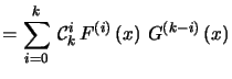
De plus, on a la formule de Leibniz : 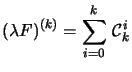
![]()
![]() avec la convention habituelle
avec la convention habituelle ![]() et
et![]() .
.
Preuve. On applique les théorèmes correspondants à chacune des coordonnées ![]() .
. ![]()
Le principe est simple, un produit scalaire, ou le produit vectoriel (dans ce cas, on est en dimension 3) se dérivent comme des produits.
Théorème : Soit ![]() , deux fonctions vectorielles de classe
, deux fonctions vectorielles de classe![]() sur
sur ![]() . Soit
. Soit ![\begin{displaymath}s:\left\{ \begin{array}[c]{rcl} I & \rightarrow & \mathbb{R... ...& F\left( x\right) G\left( x\right) \end{array} \right. \quad\end{displaymath}](img199.png)
Alors ![]() est de classe
est de classe ![]() sur
sur ![]() .
.
|
|
|
|
|
|
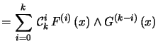
Preuve. On vérifie la formule pour ![]() .
.
Ensuite, il suffit de procéder par récurrence, comme on l'a fait lors de la dé monstration de la formule de Leibniz pour les fonctions à valeur réelle.
|
|
|
|
|
|
|
|
|
|
|
|
![]()
Théorème : Soit ![]() , deux fonctions vectorielles de classe
, deux fonctions vectorielles de classe![]() sur
sur ![]() . Soit
. Soit ![\begin{displaymath}V:\left\{ \begin{array}[c]{rcl} I & \rightarrow & \mathbb{R... ...t( x\right) \wedge G\left( x\right) \end{array} \right. \quad\end{displaymath}](img211.png)
Alors ![]() est de classe
est de classe ![]() sur
sur ![]() .
.
|
|
|
|
|
|
Preuve. On vérifie la formule pour ![]() .
.
Ensuite, il suffit de procéder par récurrence.
|
|
|
|
|
|
|
|
|
|
|
|
![]()
En résumé, dans tous les cas, un produit se dérive comme un produit.